An interesting paper demonstrating an interpretable method for deep vision models was implmented in PyTorch for a project I did in Spring 2021.
A note ahead of time: all equations and images are from the original paper (v4) unless otherwise specified.
Obviously, all credit goes to the authors.
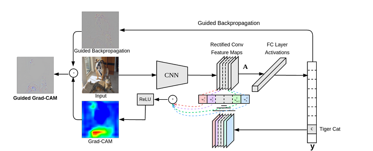
This method is termed GradCAM, and is used to highlight the convolved (or activated) features that contribute greatest to a model’s classification of an input image.
Because the regions that most siginficantly contribute to the classification are highlighted, the practitioner can infer where, for example, a model might mistake one class for another.
Just to give some context:
In order to render the mathematics intuitive, I first explain the concepts employed from a bird’s eye view, and then will briefly explain the formulae and their respective purposes described in the paper.
I will also include some code that corresponds to such an implementation in pytorch.
If it feels like a lot, I encourage the reader to pause and consider it in the context of the other things talked about here.
It can help to remind ourselves that these concepts do not exist in a vacuum.
## Historical Context For some historical context (an important thing to be sure), this paper was pushed to arxiv 3 years after Alex Krizhevsky, Ilya Sutskever, and Geoffrey Hinton debuted AlexNet on the image net challenge (ILSVRC). If ReLU is a new word, it stands for Rectified Linear Unit. There are tons of resources discussing them online.
These were very important to an idea termed Guided Backpropagation. Basically, the gradient is also passed through a ReLU function. This then leaves all neurons that positively contribute to a class’s classification. (the unit, in ReLU, refers to the neuron, which can also be referred to as a unit).
ReLU is the key ingredient to Guided Back Propagation ReLU were quickly adopted as the primary nonlinearity since it is computationally easy and has nice properties despite being on differentiable at zero. Geoffrey Hinton has an interesting lecture explaining the robustness and properties of the ReLU activation here, from around the time Alexnet won the imagenet competition in 2012. At any rate, ReLU quickly became the de facto deep learning activation for the time. Deep vision models that were equipt with the ReLU nonlinearity could immediately employ this method. The basic idea is to pass the error gradient (the residual ) through a ReLU as well. This does, however, require buffering the forward pass information (namely, the preimage of the activaions for the target layer, and all layers between it and the output layer, i.e. the classification) Some cool context for the gradient. What is it?
For the more casual reader, a gradient is a vector of all first order, explicit partial derivatives of the function.
Maybe that isnt so casual.
Here is a good explanation (also calculus, early transcendentals by Jon is a great reference)
Geometrically, it is a vector that points in the direction of the greatest rate of change of a function’s surface. Since we optimize our models to minimize error, the negative of this vector points in the exact opposite direction of the greatest change, i.e. the greatest negative rate of change. I might make a post describing this in better terms when I am a little more mathematically mature, but there are tons of great resources.
Back to our paper CAM stands for the Class Activation Map, and was a prior state of the art in interpretability. The contribution of the GradCAM paper is that it generalizes the concept and renders it agnostic to modality, in a sense. How? A score is created first through a procedure termed Global Average Pooling, where the inputs under the convolution (equivalently, the feature maps ).
Here, the CAM is weighted by the gradient of the class with respect to the feature maps.
Note the global average pooling still being used.
Why is this done, you may ask? Information between all of the features maps is shared when it is pooled in this way. Once this information is shared
Guided GradCam further extends the application of this, though it is a distinct method. It uses an elementwise muliticplication. You might wonder 1) why is this differet? 2) how does that work? To answer the former, the raw pixel value can be elementwise multiplied by corresponding entry in our GradCAM matrix. This is impossible without the matrices being the same size though. So, the authors make the GradCAM matrix the same size as the image! This is done through something called Bilinear Interpolation.
After performing this bilinear interpolation, the matrices are the same saize, and elementwise multiplication is possible.
(Another aside for the curious: The elementwise multiplication of two matrices is termed the Hadamard Product.)
The pixel values are scaled by their importance factor.
However, they are no longer bounded between 0 and 255, but no matter!
Many image libraries offer automatic normalization.
If one maps from this subset of the nonnegative reals to [0,1], one may scale these up again by the target discretization [0, 255] where non-integers are floored.
Symbolically, .
This target value needn’t overwrite the pixel values either. Instead, one image can overlay the other, and the alpha value can adjust the opacity of this filter describing the intensity of activation.
Aside: Bilinear Interpolation
Guided GradCAM: High Fidelity classwise discriminative attribution